Destructive pass/fail testing of batches

An important caveat: This post is intended as a thought exercise rather than a professional recommendation. At a later date I might return to the topic of when the methods here could be applied in the real world.

In particular, for this post, I assume that an unknown source of contamination is consistent enough to be modeled as a sequence of independent and identically distributed events. This would imply that the probabilistic contamination model can be calibrated at one time and make meaningful predictions at future times. In reality, this assumption can easily be violated. For example, if a piece of equipment breaks and introduces a new source of contamination.

For good process control, an unknown contamination source should be identified and monitored if not controlled or eliminated. Otherwise, the assumption of a consistent contamination rate can easily be wrong. Nonetheless, for this thought exercise, I'll go ahead with the assumption. I can return later to investigate how the risky assumption might be checked, perhaps by periodic recalibration.

If you produce a bad batch, and the batch isn’t well-mixed, you might have to take multiple samples from the batch to find one that fails a test. This might happen if a batch of material is contaminated, but the contaminant is not uniformly distributed within the batch. Although it would be preferable to produce no bad batches, it is possiblee to filter out bad batches with some level of reliability and confidence using process data. The simplest way would be to calculate reliability and confidence for each batch from scratch as shown in a previous post.

However, this can require many samples. Wouldn’t it be nice if we could use our observations of the contamination events to inform the sampling plan? For example, if a contamination process always results in highly detectable, homogeneous contamination, then we need fewer samples to detect a bad batch.

If you assume that the process (including contamination) is consistent over time, then you could measure the contamination at one time, and use a calibrated model to inform your batch testing protocol.

Consider a process that produces batches which are either good or bad.

Good batches always give good samples.
Bad batches sometimes give bad samples.

The batches aren’t well mixed, so a bad batch can have some good samples and some bad samples. It may be necessary to take multiple samples from a batch to determine whether it is good or bad.

How many good samples are needed before a batch has a certain probability of being good, conditional on our contamination model? Before we answer this question, I define the process more formally.

Abstraction of a process with bad batches

Variable	Description
\(N\)	Number of batches
\(i\)	Batch index
\(d_i\)	Indicator that batch \(i\) is bad
\(n_i\)	Number of samples from batch \(i\)
\(k_i\)	Number of bad samples from batch \(i\)
\(y_b\)	Probability that a batch is bad
\(y_s\)	Probability that a sample from a bad batch is bad

A process generates samples in batches. There is a probability \(y_b\) that a batch can have bad samples. Given that a batch with index \(i \in \{1, \cdots, N\}\) is bad (\(d_i = 1\)), there is a probability \(y_s\) that each sample in that batch will be bad. For a bad batch with index \(i \in \{1, \cdots, N\}\) and \(n_i\) samples, the number of bad samples \(k_i\) will have the following distribution.

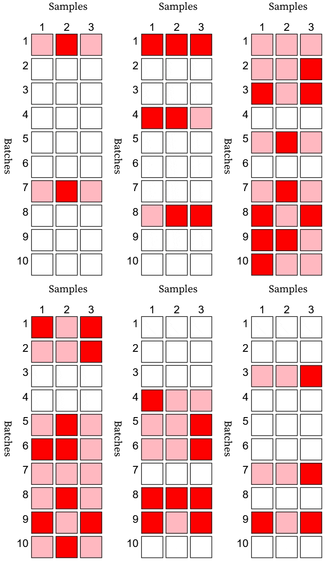
\[k_i \begin{cases} \sim \text{Binomial}(n_i, y_s)& \text{if } d_i = 1\\ = 0, & \text{if } d_i = 0 \end{cases}\]

where \(d_i\) is one or zero for a bad or good batch, respectively. You can find a visual representation of this process in an Observable notebook. In the example animation below, a bad batch appears as a pink/red row, and a good batch appears as a white row. Detecting a bad batch requires observation of a bad sample (red). If a bad batch has all good samples (pink), then it goes undetected.

Reliability with beta plot

The testing process (with perfect sensitivity and selectivity) randomly tests \(n\) samples from each batch and discards the batch if a bad sample is found. The reliability follows.

\[R = \frac{1 - y_b}{1 - y_b(1 - (1 - y_s)^n)}\]

The numerator is the fraction of good batches, and the denominator is the fraction of batches which survive inspection of \(n\) samples, whether bad or good. Our goal in batch testing is to test the fewest number of samples while ensuring reliability exceeds a desired value with a desired confidence.

\[\begin{aligned} & \text{minimize} & & n \\ & \text{subject to} & & \text{Pr}(R \geq \text{Reliability}) \geq \text{Confidence} \end{aligned}\]

To determine \(n\), we need to learn something about \(y_b\) and \(y_s\). For that, we need statistical inference from contamination data, and I will show how this can be done in a future post.