Reliability and confidence from pass/fail data
If a process sometimes fails, we can use our observations of the number of passes and failures to guarantee with some level of confidence that the fraction of non-failures is at least some reliability.
Is this the right method?
Reliability of a process is the fraction of trials that meet specifications. To limit risk, we wish to make assurances that reliability is at least some value, with a certain level of confidence. Depending on the application, practitioners will choose a desired reliability and confidence that reduces the risk of failure to an acceptable level. Given experimental data, we can calculate the reliability at our confidence level and compare it to the desired reliability.
The specifications define controlled variables and their acceptable values. If the controlled variable is not simply a binary pass/fail outcome, there are methods that benefit from the numerical information that a continuous or non-binary discrete variable has. The methods that follow only use the pass/fail determination, so they cannot benefit from knowledge of how close the outcome is to passing or failing. This makes them less efficient than methods which use fully numerical data. If your data is pass/fail, or you wish to treat data simply as pass/fail, then the rest of this post is for you.
Calculating reliability from data at a given confidence level
The reliability at a confidence level can be calculated from pass/fail data with the inverse of the cumulative beta probability density function. You can perform this calculation in LibreOffice Calc, Microsoft Excel, or Google Sheets with the following formula.
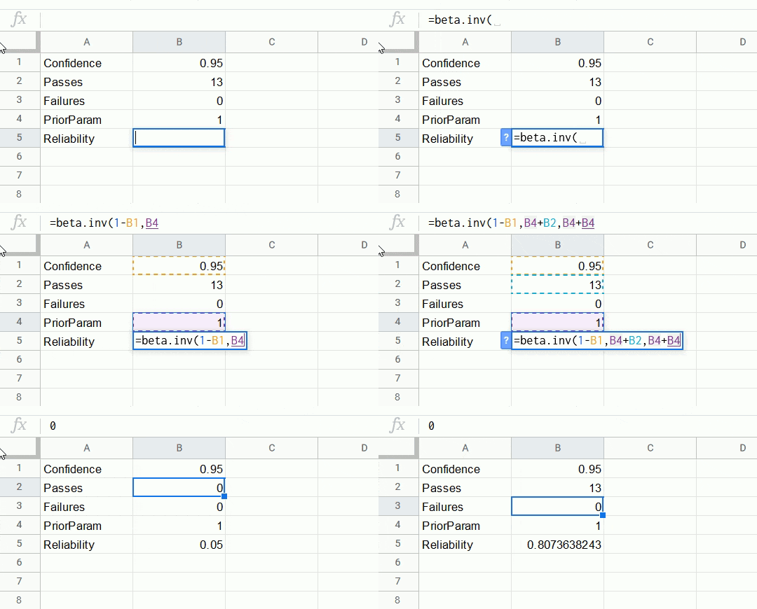
=BETA.INV(1 - Confidence, PriorParam + Passes, PriorParam + Fails)
Confidencein the above formula is the desired confidence level.Passesis the number of passing samples.Failsis the number of failing samples.PriorParamis a parameter between 0 and 1 which specifies the Bayesian prior distribution of reliability. This value represents our belief about the value of reliability in the absence of the pass/fail data. A value of 1 gives a uniform distribution between 0 and 1 in the absence of data.
With this Excel formula, one could set Confidence to the desired level, set Fails to zero, and increment Passes until the desired reliability is reached. This would give the minimum sample size, or the number of passing samples required (with no failures) to prove the desired reliability with the desired confidence.
Example. We wish to say with 95% confidence that the remote start button will activate a car with 80% reliability. In other words, for every 5 times we press the remote start button, the car should activate at least 4 times on average, and we wish to say this with 95% confidence. The minimum number of trials required in this case is 13, as shown in the gif below.

To be more conservative, we could instead take PriorParam to be zero, which gives 14 as the minimum number of trials.
Success-run theorem
There is a simpler way to calculate the minimum number of trials \(n\), which is the success-run theorem.
\[n = \frac{\log(1 - \text{Confidence})}{\log(\text{Reliability})}\]This formula can be derived from the Bayesian posterior distribution of reliability given zero failures and \(n\) successes. I will leave the derivation to another post to avoid cluttering this one.
We can plug in the numbers from our example above, and rounding up we see that we directly calculate a minimum number of samples of 14.
Beta distribution
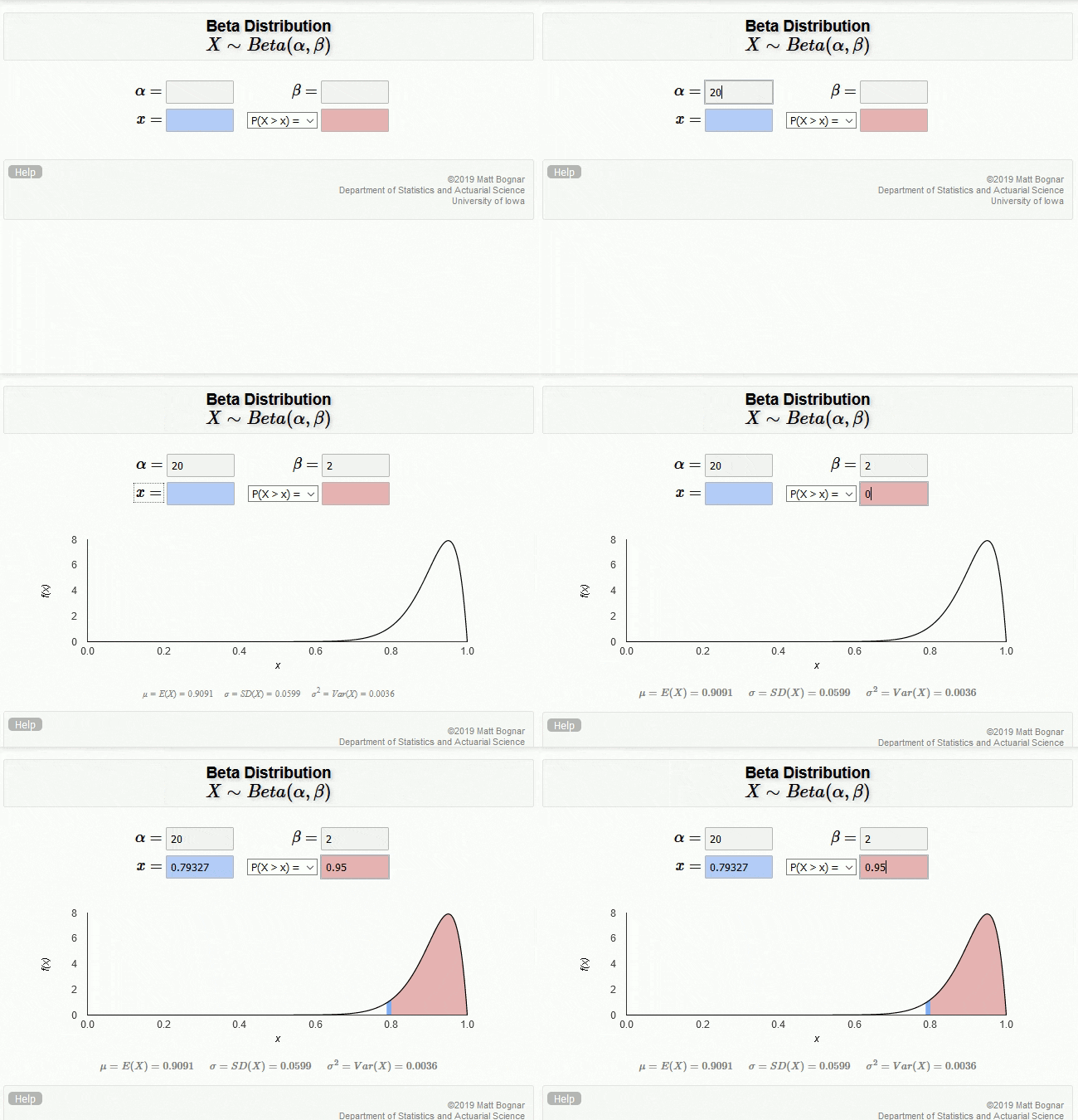
The underlying math uses the beta distribution, a probability density function defined on the interval between 0 and 1. In Bayesian statistics, this distribution can represent our certainty about the true value of reliability, because reliability also takes values between 0 and 1. An interactive plot created by Matt Bognar at the University of Iowa is useful for building intuition. Parameters \(\alpha\) and \(\beta\) of the beta distribution can be set as shown with spreadsheet applications above.
\[\alpha = \text{Passes} + \text{PriorParam}\] \[\beta = \text{Fails} + \text{PriorParam}\]Notice that if \(\alpha = \beta = 1\), the distribution is uniform between 0 and 1. By adding the number of passes and fails to \(\alpha\) and \(\beta\), respectively, we can update our belief about the true value of reliability. The gif below shows the case where we set the number of passes to 19 and number of failures to 1 (with \(\text{PriorParam}\) set to 1).

A confidence of 0.95 is entered into the bottom-right text box, which populates the bottom-left text box with the reliability (0.79) and draws the confidence as the integral of the distribution, filled in above the reliability level.
By playing with the values of \(\alpha\) and \(\beta\), you can get a sense for how the distribution changes with additional data. Notice how the mean of the distribution is \(\frac{\alpha}{\alpha + \beta}\), and the width of the distribution decreases as the amount of data increaes.
A useful approach given binary data
For each failure mode of a process, a minimum reliability with some confidence should be decided based on a risk assessment. Once the risk assessment is done, one can use the approach shown here to test whether pass/fail data is consistent with the desired reliability and confidence. This is done by checking that the desired reliability is exceeded by the computed, inferred reliability, as demonstrated with the BETA.INV function earlier.